Wiki
Table of Contents
📚 General options
The following parameters are common when running phabox2:
--task
    Select a program to run:
    end_to_end    || Run phamer, phagcn, phatyp, and cherry once (default)
    phamer        || Virus identification
    phagcn        || Taxonomy classification
    phatyp        || Lifestyle prediction
    cherry        || Host prediction
    phavip        || Protein annotation
    contamination || Contamination/proviurs detection
    votu          || vOTU grouping (ANI-based or AAI-based)
    tree          || Build phylogenetic trees based on marker genes

--contigs
    Path of the input FASTA file (required)

--proteins
    FASTA file of predicted proteins. (optional)

--len
    Filter the length of contigs || default: 3000
    Contigs with length smaller than this value will not proceed
📚 Special options
Please note that end_to_end task will run phamer, phagcn, cherry, phatyp, and phavip together. Thus, each task's options can also be used for the end_to_end task.
In addition, prediction with non-virus and low-confidence will not be used in the following taxonomy, host, and lifestyle prediction tasks.
The following parameters will be used in specific tasks:
📕 PhaMer (Virus identification)
In-task options:
--reject
    Reject sequences in which the percent proteins aligned to known phages is smaller than the value.
    Default: 10
    Range from 0 to 20
If the proportion is too low, the prediction for downstream analysis will be unreliable.
📕 PhaGCN (Taxonomy)
In-task options:
The options below are used to generate a network for virus-virus connections. The current parameters are optimized for the ICTV 2024 and are highly accurate for grouping genus-level vOTUs. When making changes, make sure you understand 100% what they are.
--aai
    Average amino acids identity  || default: 75 || range from 0 to 100

--share
    Minimum shared number of proteins || default: 15 || range from 0 to 100

--pcov
    Protein-based coverage || default: 80 || range from 0 to 100

--draw (local version only)
    Draw network examples for the query virus relationship. || default: N || Y or N
--draw is used to plot sub-networks containing the query virus. We use it to generate visualization for our web server. However, it will only print the top 10 largest sub-networks, so we do not recommend that users use it. We have provided the complete network for visualization (network_edges.tsv and network_nodes.tsv file) please check it out via: here
📕 CHERRY (Host)
In-task options:
The options below are used to generate a network for virus-virus connections. The current parameters are optimized for the ICTV 2024 and are highly accurate for grouping genus-level vOTUs. When making changes, make sure you understand 100% what they are.
--aai
    Average amino acids identity  || default: 75 || range from 0 to 100

--share
    Minimum shared number of proteins || default: 15 || range from 0 to 100

--pcov
    Protein-based coverage || default: 80 || range from 0 to 100

--draw (local version only)
    Draw network examples for the query virus relationship. || default: N || Y or N
--draw is used to plot sub-networks containing the query virus. We use it to generate visualization for our web server. However, it will only print the top 10 largest sub-networks, so we do not recommend that users use it. We have provided the complete network for visualization (network_edges.tsv and network_nodes.tsv file) please check it out via: here
The options below are used to align contigs to CRISPRs.
--cpident
    Alignment identity for CRISPRs || default: 90 || range from 90 to 100

--ccov
    Alignment coverage for CRISPRs || default: 90 || range from 0 to 100

--blast (local version only)
    BLAST program for CRISPRs || default: blastn || blastn or blastn-short
    blastn-short will lead to more sensitive results but require more time to execute the program
The default parameters are optimized for predicting prokaryotic hosts for the virus with 98% accuracy (data from the NCBI RefSeq database). When making changes, make sure you understand 100% what they are.
📕 PhaTYP (Lifestyle)
In-task options:
There are no additional options for lifestyle prediction. Only need to follow the general options.
📕 PhaVIP (annotation)
Please note that running task end_to_end, phamer, phagcn, phatyp, and cherry, will automatically run phavip. The output files are the same.
In-task options:
--sensitive (local version only)
    Sensitive when search for the prokaryotic genes || default: N ||  Y or N
    Y will lead to more sensitive results but require more time to execute the program
📗 Contamination
In-task options:
There are no additional options for lifestyle prediction. Only need to follow the general options.
📘 vOTU grouping
In-task options:
--mode
    Mode for clustering ANI based or AAI based || default: ANI || ANI or AAI
AAI-based options:
--aai
    Average amino acids identity for AAI based genus grouping || default: 75 || range from 0 to 100

--pcov
    Protein-level coverage for AAI based genus grouping || default: 80 || range from 0 to 100

--share
    Minimum shared number of proteins for AAI based genus grouping || default: 15 || range from 0 to 100
ANI-based options:
--ani
    Alignment identity for ANI-based clustering  || default: 95 || range from 0 to 100

--tcov
    Alignment coverage for ANI-based clustering || default: 85 || range from 0 to 100
📙 Pylogenetic tree
In-task options:
--marker
    A list of markers used to generate tree || default: terl portal
    You can choose more than one marker to generate the tree from below:

    The marker genes were obtained from the RefSeq 2024:
        endolysin      || 91% prokaryotic virus have endolysin
        holin          || 75% prokaryotic virus have holin
        head           || 77% prokaryotic virus have marjor head
        portal protein || 84% prokaryotic viruses have portal
        terl           || 92% prokaryotic viruses have terminase large subunit

        Using combinations of these markers can improve the accuracy of the tree
        But will decrease the number of sequences in the tree.

--mcov
    Alignment coverage for matching marker genes || default: 50 || range from 0 to 100

--mpident
    Alignment identity for matching marker genes || default: 25 || range from 0 to 100

--msa (local version only)
    Whether run msa || default: N || Y or N
    Y will run msa for the marker genes using mafft
    But this will require more time to execute the program

--tree (local version only)
    Whether build a tree || default: N || Y or N
    Y will generate the tree based on the marker genes using FastTree
    But this will require more time to execute the program
Table of Contents
- 📕 Virus identification
- 📕 Taxonomy classification
- 📕 Host prediction
- 📕 Lifestyle prediction
- 📕 Protein annotation
- 📚 End to end task
- 📗 Contamination
- 📘 vOTU grouping
- 📙 Phylogenetic tree
All the outputs can be found in the PATH_TO_OUT/final_prediction/ folder. According to the --task you run, the total number of files may differ.
📕 PhaMer (Virus identification)
final_prediction
├── phamer_prediction.tsv
└── phamer_supplementary
     ├── all_predicted_contigs.fa    || DNA sequences > --length
     ├── all_predicted_protein.fa    || Proteins predicted by prodigal-gv
     ├── gene_annotation.tsv         || protein annotation based on blastp
     ├── predicted_virus.fa          || Vrial DNA sequences
     ├── predicted_virus_protein.fa  || Vrial proteins
     ├── alignment_results.tab       || blastp results against db
     └── uncertain_sequences_for_contamination_task.fa      || please run contamination task
The main output phamer_prediction.tsv is generated in tabular-separated (TSV) format composed of six fields:
Accession       Length  Pred    Proportion      PhaMerScore     PhaMerConfidence
example_0       29445   virus   0.1             1.0             lower than reject threshold
example_2       5971    virus   0.86            1.0             high-confidence
- Accession: the accession or the name of the input contigs.
- Length: the length of input contigs.
- Pred: virus or non-virus.
- Proportion: the proportion of the proteins that can be aligned to the virus database (from 0 to 1).
- PhaMerScore: the prediction score given by the deep learning model.
- PhaMerConfidence: the confidence of prediction, determined by both Proportion and PhaMerScore.
- high-confidence
- medium-confidence
- low-confidence
- lower than viral score threshold.
- lower than reject threshold (according to the --reject parameter, default: 0.1).
For the virus with low-confidence or lower than viral score threshold, we recommend you to run the --task contamination to check their sequence quality.
📕 PhaGCN (Taxonomy)
final_prediction
├── phagcn_prediction.tsv
└── phagcn_supplementary
   ├── all_predicted_contigs.fa   || DNA sequences > --length
   ├── all_predicted_protein.fa   || Proteins predicted by prodigal-gv
   ├── alignment_results.tab      || blastp results against db
   ├── gene_annotation.tsv        || protein annotation based on blastp
    ├── phagcn_network_edges.tsv   || network file for cytoscape
    └── phagcn_network_nodes.tsv   || network file for cytoscape
The main output phagcn_prediction.tsv is generated in tabular-separated (TSV) format composed of six fields:
Accession       Length  Lineage PhaGCNScore     Genus   GenusCluster
example_0       29445   superkingdom:Viruses;clade:Duplodnaviria;kingdom:Heunggongvirae;phylum:Uroviricota;class:Caudoviricetes 1.00;1.00;1.00;1.00;1.00;1.00;0.58;0.58 -       singleton
example_103     11376   superkingdom:Viruses;clade:Duplodnaviria;kingdom:Heunggongvirae;phylum:Uroviricota;class:Caudoviricetes;genus:Jasminevirus      1.00;1.00;1.00;1.00;1.00;1.00;1.00      Jasminevirus      known_genus
- Accession: the accession or the name of the input contigs.
- Length: the length of input contigs.
- Lineage: the predicted taxonomy lineage (NCBI version) of the contigs. Each rank is separated by the ';'.
- PhaGCNScore: the predicted score for each rank in the lineage. Each rank is separated by the ';'.
- Genus: whether the contig has a genus level name ('-' means unknown).
- GenusCluster: if the Genus is '-', the program will assign a genus-level grouping result: group_idx (idx = 1, 2, 3, ...) or singleton. This can be viewed as genus-level OTUs based on the average shared protein identities between sequences.
📕 CHERRY (Host)
final_prediction
├── cherry_prediction.tsv
└── cherry_supplementary
    ├── all_predicted_contigs.fa   || DNA sequences > --length
    ├── all_predicted_protein.fa   || Proteins predicted by prodigal-gv
    ├── alignment_results.tab      || blastp results against db
    ├── gene_annotation.tsv        || protein annotation based on blastp
    ├── cherry_network_edges.tsv   || network file for cytoscape
    └── cherry_network_nodes.tsv   || network file for cytoscape
The main output cherry_prediction.tsv is generated in tabular-separated (TSV) format composed of five fields:
Accession       Length  Host                                            CHERRYScore     Method
example_99      6612    species:Halobiforma_lacisalsi                   1.00            CRISPR-based (DB)
example_98      13996   species:Salinispora_arenicola                   1.00            CRISPR-based (DB)
- Accession: the accession or the name of the input contigs.
- Length: the length of input contigs.
- Host: the predicted host (NCBI taxonomy) of the contigs. '-' means unknown host.
- CHERRYScore: the predicted score from the model.
- Method:
- CRISPR-based(MAG): CRISPRs alignment results from provided MAG (if any)
- CRISPR-based(DB): CRISPRs alignment results from database.
- AAI-based: predicting host based on virus-similarity
📕 PhaTYP (Lifestyle)
final_prediction
├── phatyp_prediction.tsv
└── phatyp_supplementary
    ├── all_predicted_contigs.fa   || DNA sequences > --length
    ├── all_predicted_protein.fa   || Proteins predicted by prodigal-gv
    ├── alignment_results.tab      || blastp results against db
    └── gene_annotation.tsv        || protein annotation based on blastp
The main output phatyp_prediction.tsv is generated in tabular-separated (TSV) format composed of four fields:
Accession       Length  TYPE            PhaTYPScore
example_0       29445   virulent        1.0
example_2       5971    temperate       1.0
- Accession: the accession or the name of the input contigs.
- Length: the length of input contigs.
- TYPE: virulent or temperate (virus).
- PhaTYPScore: the prediction score given by the deep learning model.
📕 PhaVIP (Protein annotation)
Please note that running task end_to_end, phamer, phagcn, phatyp, and cherry, will automatically run phavip. The output files are the same.
final_prediction
└── phavip_supplementary
    ├── all_predicted_contigs.fa   || DNA sequences > --length
    ├── all_predicted_protein.fa   || Proteins predicted by prodigal-gv
    ├── alignment_results.tab      || blastp results against db
    └── gene_annotation.tsv        || protein annotation based on blastp
The main output gene_annotation.tsv is generated in tabular-separated (TSV) format composed of four fields:
Genome  ORF     Start   End     Strand  GC      Annotation
example_0 example_0_1       347     790     1       0.619   hypothetical protein
example_0 example_0_2       790     1944    1       0.591   hypothetical protein
example_0 example_0_3       2454    2627    1       0.58    capsid accessory protein
- Genome: the accession or the name of the input contigs.
- ORF: the ID of the translated protein.
- Start: start position on the genome./li>
- End: end position on the genome.
- Strand: forward (1) or backward(-1).
- GC: GC content.
- Annotation: protein annotation.
📚 End to end task
final_prediction
├── final_prediction_summary.tsv
├── phamer_supplementary
│   ├── all_predicted_contigs.fa
│   ├── all_predicted_protein.fa
│   ├── gene_annotation.tsv         || outputs of phavip
│   ├── predicted_virus.fa
│   ├── predicted_virus_protein.fa
│   ├── alignment_results.tab
│   └── uncertain_sequences_for_contamination_task.fa      || please run contamination task
├── phagcn_supplementary
│   ├── phagcn_network_edges.tsv
│   └── phagcn_network_nodes.tsv
├── cherry_supplementary
│   ├── cherry_network_edges.tsv
│   └── cherry_network_nodes.tsv
└── phatyp_supplementary
In the end-to-end mode, except for the aforementioned xxx_prediction.tsv files, a final_prediction_summary.tsv is generated by merging the outputs of all subprograms.
In addition, prediction with non-virus and low-confidence will not be used in the following taxonomy, host, and lifestyle prediction tasks.
📗 Contamination
final_prediction
├── contamination_prediction.tsv
└── contamination_supplementary
    ├── proviruses.fa                              || proteinal provirues
    ├── candidate_provirus.tsv                     || information of the provirus
    └── marker_gene_from_contamination_search.tsv  || marker gene annotation
The main output contamination_prediction.tsv is generated in tabular-separated (TSV) format composed of nine fields:
Accession      Length   Total_genes  Viral_genes  Prokaryotic_genes  Kmer_freq  Contamination  Provirus   Pure_viral
example_270    6617            6            2            0           1.0        0              No         High quality
example_271    17630           28           9            0           1.0        0              No         High quality
- Accession: the accession or the name of the input contigs.
- Length: the length of input contigs.
- Total_genes: number of genes in the contigs (predicted by prodigal-gv)
- Viral_genes: number of viral marker genes
- Prokaryotic_genes: number of prokaryotic marker genes
- Kmer_freq: average frequency of 20-mer.
- This is a value to estimate the copy number of the genes; usually, the Kmer_freq of 99.9% virus is less than 1.25.
- Contamination:
- Provirus: Whether the sequence is a provirus
- Pure_viral: High quality or Medium quality or Low quality
📘 vOTU grouping
final_prediction
├── ANI_based_vOTU.tsv (ANI-based)
└── AAI_based_vOTU.tsv (AAI-based)
The main output xxx_based_vOTU.tsv is generated in tabular-separated (TSV) format composed of four fields:
Sequence        vOTU            Representative  Length
contig_33       group_19        contig_33       49448
contig_34       group_19        contig_33       4484
- Accession: the accession or the name of the input contigs.
- vOTU: the cluster ID.
- Representative: the representative genome.
- Length: the length of input contigs.
📙 Phylogenetic tree
final_prediction
├── combined_marker.msa (if msa =='Y')    || concatenate the MSA between different marker (local version only)
├── combined.tree (if tree == 'Y')        || phylogenetic tree based on FastTree (local version only)
└── tree_supplementary
    └── finded_marker_xxx_combined_db.fa  || the fined marker and database marker
    └── finded_marker_xxx_without_db.fa  || the found marker without database marker
Table of Contents
Some outputs from PhaBOX can help you to draw figures for your research. We will show some examples below. Hope they will help
📘 Portein visualization
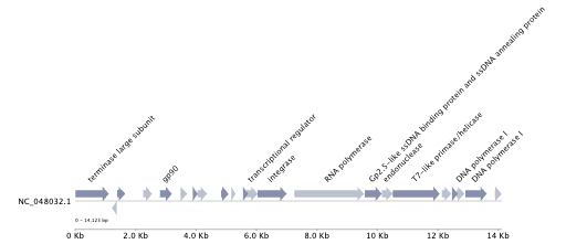
The protein annotation file gene_annotation.tsv can be used to generate the protein organization using PyGenomeViz.
# Make sure you have installed the PyGenomeViz
# pip install pygenomeviz

#Load the data
import pandas as pd
data = pd.read_csv('gene_annotation.tsv', sep='\t')

# Convert your data into a format suitable for pygenomeviz. You need to extract relevant information:
# Extract the relevant columns
annotations = []
for index, row in data.iterrows():
    annotations.append({
        'seq_id': row['Genome'],
        'start': row['Start'],
        'end': row['End'],
        'strand': row['Strand'],
        'annotation': row['Annotation'],
    })

from pygenomeviz import GenomeViz
# Initialize GenomeViz
gv = GenomeViz()
# Add each annotation as a track
for ann in annotations:
    gv.add_feature(
        seq_id=ann['seq_id'],
        start=ann['start'],
        end=ann['end'],
        strand=ann['strand'],
        label=ann['annotation']
    )

# Render the visualization
gv.render()
# Save to a file
gv.savefig('genome_viz.png')
# Or display it
gv.show()
An example is:
| Genome Annotation |
 |
📘 Network visualization
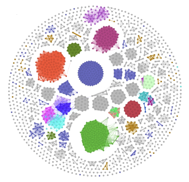
The network files xxx_edges.csv and xxx_nodes.csv can be used to input into Cytoscape.
Step1 Import the network:
  - Go to File > Import > Table from File
  - select xxx_edges.csv
Step2 Import the network:
  - Go to File > Import > Table from File
  - select xxx_nodes.csv
Setp3 Adjust the visualization:
  - choose a layout
  - color the nodes
An example is:
| Network Visualization |
 |
📘 Tree visualization
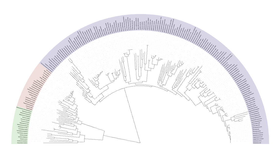
The tree file combined.tree can be used as input to iTOL. The metadata of the reference genomes can be found in PhaBOX2's database RefVirus.csv.
An example is:
| Tree Visualization |
 |
